DuckDB Tutorial: Data Analysis with CLI and Python API

This is a comprehensive hands-on guide to using the DuckDB database to perform a real-world data project in a containerized workspace using Daytona.

You’ll follow me from setup to working with DuckDB CLI and even with Python via its Client API. So it’s a long ride, and you can get a coffee nearby.

This comprehensive guide will teach you how to prepare personal loan marketing campaign data for importation into a DuckDB database and analyze the dataset. Your tasks will include collecting and reviewing the data, cleaning and structuring it according to a specification, handling errors and inconsistencies, and transforming and splitting it into multiple CSV files.

The CSV file you’ll work on is called bank_marketing.csv. Download from GitHub here.

Prerequisites

To follow along with a hands-on guide about DuckDB Playground in Daytona, you’ll need to have the following;

• An IDE (It could be VS Code or JetBrains) or just a terminal.

• Docker installation on your PC or Mac. Click here for more info.

• Daytona installation on your PC or Mac. Click here for more info.

• A GitHub account to create a repository. The link here is to create one if you don’t have one.

• Basic knowledge of Git and GitHub.

What’s DuckDB and Why Use it

DuckDB is a fast in-process data analytical database that supports a feature-rich SQL dialect and deep integrations into client APIs. It’s designed to perform highly complex queries against large databases in embedded configuration, such as combining tables with hundreds of columns and billions of rows. It’s specialized for online analytical processing (OLAP) workloads.

DuckDB has many features that make it stand out among other databases focusing on OLAP. Some of the features are:

• Simple: It’s straightforward to install and perform embedded in-process operations.

• Portable: Since it has no external dependencies, it’s extremely portable and can be compiled for all major operating systems and CPU architectures.

• Feature-Rich: DuckDB has some interesting features, such as extensive support for SQL complex queries, integrations with languages like Python, R, and Java, and the ability to store data as persistent, single-file databases.

• Speed: It’s faster because it uses a columnar-vectorized query execution engine, which improves performance when running OLAP workloads.

• Free: Lastly, it’s a free open-source database system, which anyone can use because of its permissive MIT License.

Setting up Daytona Workspace for DuckDB Playground

Alright, that’s enough reading. Now, let us start writing codes. You must set up a DuckDB environment in a Daytona workspace to do so. Let’s begin.

Step 1: Create a GitHub Repository

First, go to the GitHub website and create a repository using the name of your choice. For my repository, I’ll use playground-duckdb.

Step 2: Clone the repository using Git

After creating the repository, the next step is to clone it onto your local PC or Mac. To do so, open your terminal and run the command git clone https://github.com/USERNAME/REPOSITORY-NAME. Replace the placeholders with your GitHub username and the repository name you chose in step 1.

In my case, it’s a git clone https://github.com/c0d33ngr/playground-duckdb

Step 3: Prepare your devcontainer.json file and dataset in CSV format

Run the command to move into your cloned repository, but don’t forget to replace playground-duckdb with the repository name you created if yours isn’t the same as mine.

1cd playground-duckdb

Download the bank campaign dataset you are going to perform data tasks on which is in CSV format, from the GitHub repo here.

Note: It has to be in the directory of your clone repository. In my case, it’s inside playground-duckdb.

Now, let us proceed to the next step.

Create a hidden directory named .devcontainer where our devcontainer.json file will be. Let’s do so and move into it.

Run the command to do so

1mkdir .devcontainer && cd .devcontainer

Let’s create our devcontainer.json file in the .devcontainer directory.

I use nano to create my .devcontainer.json file using this command.

1nano devcontainer.json

Paste this code into your devcontainer.json file.

1{
2    "name": "DuckDB Playground",
3    "image": "mcr.microsoft.com/devcontainers/base:ubuntu",
4    "features": {
5        "ghcr.io/eitsupi/devcontainer-features/duckdb-cli:1": {},
6        "ghcr.io/devcontainers/features/python:1": {}
7    },
8    "postCreateCommand": "pip install duckdb matplotlib pandas"
9}

The devcontainer.json content contains configurations to start your DuckDB environment in a Daytona workspace.

• name: This sets the name of the development container environment to DuckDB Playground.

• image: This uses a base Ubuntu image from the Microsoft image repository.

• features: This configuration adds DuckDB installation and Python setups in the Daytona workspace

• postCreateComand: This installs the Python packages needed for this guide into the workspace.

After creating and saving the devcontainer.json file, move up back to the root directory of your clone repository. I run the command below.

1cd ../..

Step 4: Commit and Push Changes to GitHub

Run these commands to push your changes to GitHub.

1git add .
2git commit -m “add devcontainer.json file”
3git push

You have successfully pushed our updated repository containing the configuration file (devcontainer.json) for our DuckDB environment.

Step 5: Verify Daytona Installation

Run this command to check daytona is properly installed on your PC or Mac.

1daytona –-version

You should see your version of daytona installed.

Step 6: Create a Daytona Workspace with DuckDB Playground Environment in it

Let’s start the daytona server by running the command.

1daytona serve

You should see logs like my screenshot.

Please open a new tab in your terminal, for Linux its Shift + Ctrl + T

Run the command below in a new tab of your terminal and follow the prompt instructions. It would ask you for a workspace name to use; choose the default.

Replace USERNAME and REPOSITORY-NAME with your username for GitHub and the repository name you created earlier.

1daytona create https://github.com/USERNAME/REPOSITORY-NAME

In my case, it’s this.

1daytona create https://github.com/c0d33ngr/playground-duckdb

After you successfully run the above command you should see a screenshot like mine showing your Daytona workspace that contains the DuckDB environment is running.

You can now run this command to open the DuckDB environment in your default IDE you choose when installing Daytona (Replace WORKSPACE-NAME with the name you used when creating the workspace above, in my case it’s playground-duckdb).

1daytona code WORKSPACE-NAME

That’s it. Daytona will create a DuckDB playground environment for you and open it in the default IDE you set.

Using DuckDB as a Command Line Interface (CLI) Tool

In this section, you’ll learn how to work with DuckDB by creating a database from a CSV file, examining its structure, retrieving distinct values, and exporting data to separate CSV files for client, campaign, and economics data. Finally, you’ll verify the exported data, gaining hands-on experience with DuckDB’s querying and data manipulation capabilities. Let us get started.

Step 1: Enter DuckDB Interactive Shell

By now, you should be in your default IDE set up using daytona. In your IDE terminal, type the command below to enter into the DuckDB database shell in interactive mode where you’ll run some SQL-based queries that conform to the DuckDB database.

1duckdb

Step 2: Create a Database from the CSV file

Let’s create a database named bank_marketing from the CSV file you downloaded earlier. To do so, run the DuckDB SQL in the database shell.

1CREATE TABLE bank_marketing AS
2FROM 'bank_marketing.csv';

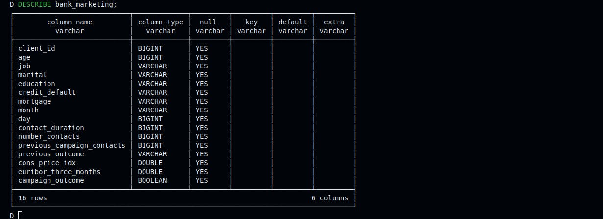
Step 3: Check the Database Structure

To check the database table schema, run this SQL in the shell.

1DESCRIBE bank_marketing;

Step 4: Export Client Data to CSV

Run the following SQL query to export client data to a CSV file named client.csv.

1COPY (
2    SELECT 
3        client_id,
4        age,
5        REPLACE(job, '.', '_') AS job,
6        marital,
7        REPLACE(education, '.', '_') AS education,
8        CASE 
9            WHEN credit_default = 'yes' THEN 1 
10            ELSE 0 
11        END AS credit_default,
12        CASE 
13            WHEN mortgage = 'yes' THEN 1 
14            ELSE 0 
15        END AS mortgage
16    FROM 
17        bank_marketing
18) TO 'client.csv' (DELIMITER ',', HEADER TRUE);

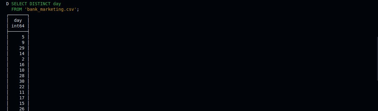
Step 5: Retrieve the List of Distinct Records in day Column

Run the following SQL query to retrieve a list of distinct days from the bank_marketing table. The results would be useful in preparing the SQL query for step 7. We need to know the unique records in the day column.

1SELECT DISTINCT day
2FROM 'bank_marketing.csv';

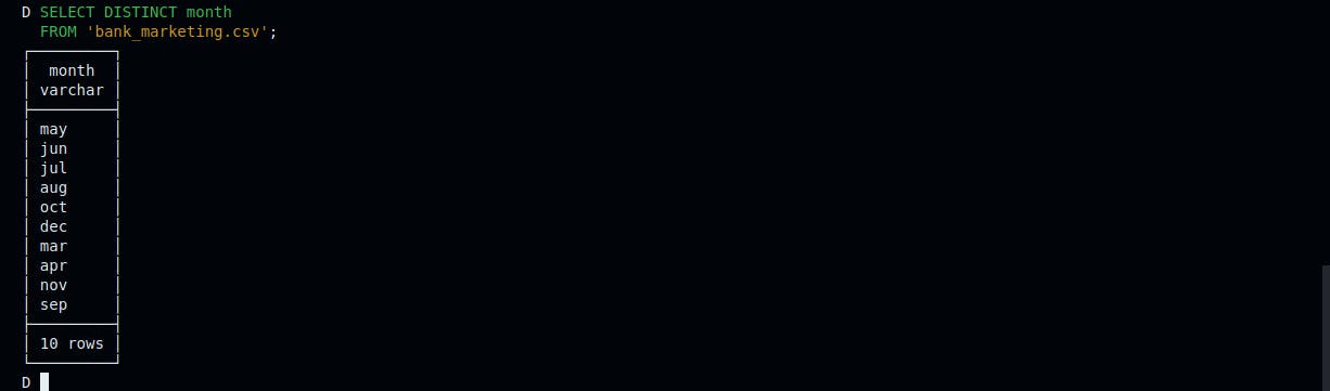
Step 6: Retrieve the List of Distinct Records in month Column

Run the following SQL query to retrieve the list of distinct months from the bank_marketing table. The results will also be needed to create a new column called last_contact_date later in step 7.

1SELECT DISTINCT month
2FROM 'bank_marketing.csv';

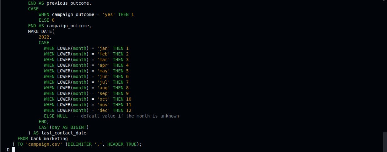
Step 7: Export Campaign Data to CSV

Run the following SQL query to export campaign data to a CSV file named campaign.csv

1COPY (
2  SELECT 
3      client_id,
4      number_contacts,
5      contact_duration,
6      previous_campaign_contacts,
7      CASE
8          WHEN previous_outcome = 'success' THEN 1
9          ELSE 0
10      END AS previous_outcome,
11      CASE
12          WHEN campaign_outcome = 'yes' THEN 1
13          ELSE 0
14      END AS campaign_outcome,
15      MAKE_DATE(
16          2022,
17          CASE 
18            WHEN LOWER(month) = 'jan' THEN 1
19            WHEN LOWER(month) = 'feb' THEN 2
20            WHEN LOWER(month) = 'mar' THEN 3
21            WHEN LOWER(month) = 'apr' THEN 4
22            WHEN LOWER(month) = 'may' THEN 5
23            WHEN LOWER(month) = 'jun' THEN 6
24            WHEN LOWER(month) = 'jul' THEN 7
25            WHEN LOWER(month) = 'aug' THEN 8
26            WHEN LOWER(month) = 'sep' THEN 9
27            WHEN LOWER(month) = 'oct' THEN 10
28            WHEN LOWER(month) = 'nov' THEN 11
29            WHEN LOWER(month) = 'dec' THEN 12
30            ELSE NULL  -- default value if the month is unknown
31          END,
32          CAST(day AS BIGINT)
33      ) AS last_contact_date
34  FROM bank_marketing
35) TO 'campaign.csv' (DELIMITER ',', HEADER TRUE);

Step 8: Export economic data to CSV

Run the following SQL query to export economics data to a CSV file named economics.csv

1COPY (
2    SELECT 
3        client_id,
4        cons_price_idx,
5        euribor_three_months
6    FROM bank_marketing
7) TO 'economics.csv' (DELIMITER ',', HEADER TRUE);

Step 9: Read Data from Exported CSV files

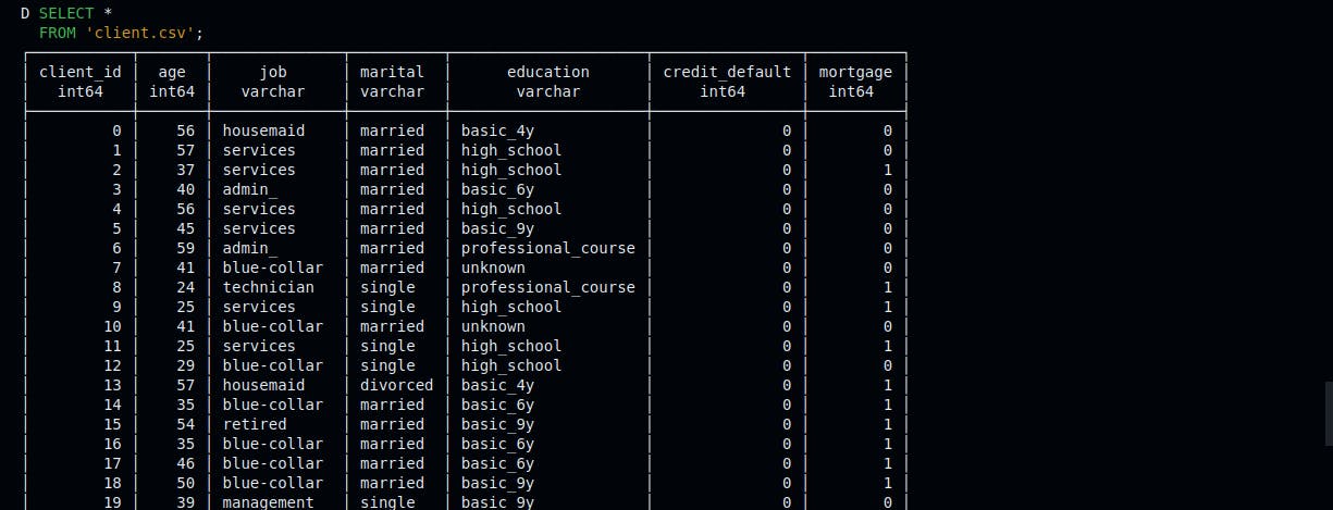
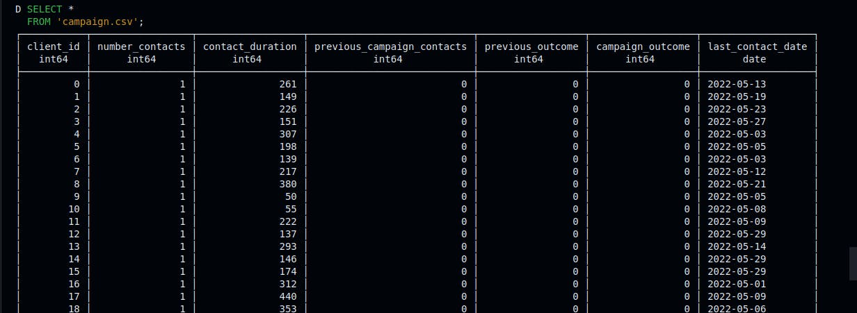
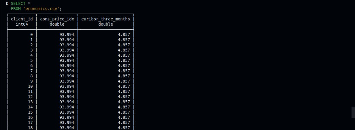
Run the following SQL queries to read data from the client.csv, campaign.csv, and economics.csv files.

1SELECT *
2FROM 'client.csv';

1SELECT *
2FROM 'campaign.csv';

1SELECT *
2FROM 'economics.csv';

Our three CSV files have been prepared for analysis using the DuckDB Client API via Python. Let’s proceed to the next section.

Using DuckDB with Python through its Client API

In this section, you’ll learn how to analyze and visualize data using DuckDB and Matplotlib. You’ll calculate the campaign success rate, create a bar chart to compare average client age by education level, and generate a scatter plot to explore the relationship between contact duration and campaign outcome. In this section, we’ll use the cleaned and transformed CSV files split from our bank_marketing.csv.

Step 1: Analysis of Customer Campaign Success Rate

Create a file name campaign_success_rate.py. Paste the following Python code in it and save.

1import duckdb
2
3result = duckdb.sql(
4    """
5    SELECT AVG(campaign_outcome) AS campaign_outcome_mean
6    FROM 'campaign.csv';
7    """
8).fetchall()
9
10success_rate = result[0][0]  # Access the value directly
11
12print(f"Campaign success rate: {success_rate:.2%}")

Run the campaign_success_rate.py file in your IDE terminal using python3 campaign_success_rate.py and see the campaign success rate of the campaign.csv output in your IDE terminal.

Step 2: Analysis and Visualization of Client Age by Educational Level

Create another file named client_age_by_education.py. Paste the following Python code in it and save.

1import duckdb
2import matplotlib.pyplot as plt
3
4result = duckdb.sql(
5    """
6    SELECT
7        education,
8        AVG(age) AS average_age
9    FROM
10      'client.csv'
11    GROUP BY
12        education
13    ORDER BY
14        education;
15    """
16).fetchdf()
17
18
19# Plot the results
20plt.figure(figsize=(8, 6))
21plt.bar(result['education'], result['average_age'])
22plt.xlabel('Education Level')
23plt.ylabel('Average Age')
24plt.title('Average Client Age by Education Level')
25plt.xticks(rotation=45)  # Rotate x-axis labels for better readability
26plt.tight_layout()
27plt.savefig('plot-1.png')

Run the file in your IDE terminal using python3 client_age_by_education.py. The visualization plot should be saved as plot-1.png.

Step 3: Analysis and Visualization of Contact Duration and Campaign Outcome Through Correlation

Lastly, create a new file named contact_duration_vs_outcome.py. Paste the following code and save it.

1
2import duckdb
3import matplotlib.pyplot as plt
4
5result = duckdb.sql(
6    """
7    SELECT 
8        contact_duration,
9        campaign_outcome
10    FROM 'campaign.csv';
11    """
12).fetchdf()
13
14
15plt.figure(figsize=(8, 6))
16plt.scatter(result['contact_duration'], result['campaign_outcome'])
17plt.xlabel('Contact Duration')
18plt.ylabel('Campaign Outcome')
19plt.title('Relationship Between Contact Duration and Campaign Outcome')
20plt.yticks([0, 1])  # Set y-axis ticks to 0 and 1
21plt.savefig('plot-2.png')

Run the file in the IDE terminal using python3 contact_duration_vs_outcome.py. You should also see another visualization plot saved as plot-2.png.

Conclusion

In this comprehensive guide, you have explored the capabilities of using DuckDB in a Daytona Workspace with no stress through hands-on examples.

Throughout this guide, you have gained practical experience in creating and managing an in-memory database with DuckDB, performing SQL queries for data cleaning, transformation, and splitting, and integrating DuckDB with Python using its Client API for data analysis.